II.8.2.1 Construction de solutions du problème dual adjoint.

Définissons d'abord les fonctions <I>E^'_kl et <I>H^'_kl (II.8.4) qui d'après la définition 14 donnent les fonctions de base ${{\mathcal{Z}}}_{kl}$ par (II.8.5). Pour cela introduisons les ondes planes de polarisations complexes que nous appellerons ``fonctions de type <I>F ou de type <I>G''.

Définition 15   Sur chaque maille $\Omega _k$ on considère p directions de propagation réelles normées V_k,l^', l'indice l^' variant de 1 à p, telles que

$$\forall (l,m) \in [1,p]^2, \ l \ne m \Longrightarrow V_{k,l} \ne V_{k,m} \ .$$ (II.8.20)

Pour une direction de propagation V_k,l^' donnée, on choisit un vecteur polarisation réel et normé <I>E⁰_k,l^', quelconque dans le plan orthogonal à la direction de propagation V_k,l^'. Ce vecteur réel <I>E⁰_k,l^' définit les polarisation complexes <I>F_k,l^' et <I>G_k,l^' par

$$\null\,\vcenter{\openup\jot \let\\ =\@ \ialign{\strut\hfil$... ...E}}^{0}_{k,l^{'}} \wedge V_{k,l^{'}} \right) \ . \cr \crcr}}\,$$ (II.8.21)

On définit alors deux fonctions <I>E^<I>F_k,l^' et <I>E^<I>G_k,l^':

1. la fonction <I>E^<I>F_k,l^' par
   

   $${{\mathbf E}}^{{{\mathbf F}}}_{k,l^{'}}=\sqrt{\overline{\mu}... ...}_{k}}\left({V_{k,l^{'}}} \, . \, {{{\mathbf X}}}\right) } \ ,$$ (II.8.22)

   
   

2. la fonction <I>E^<I>G_k,l^' par
   

   $${{\mathbf E}}^{{{\mathbf G}}}_{k,l^{'}}=\sqrt{\overline{\mu}... ...}_{k}}\left({V_{k,l^{'}}} \, . \, {{{\mathbf X}}}\right) } \ .$$ (II.8.23)

   
   

Les fonctions <I>E^<I>F_k,l^' et <I>E^<I>G_k,l^' sont étendues à tout le domaine $\Omega$ par la fonction nulle

$$% j \ne k \Longrightarrow \left\{ \null\,\vcenter{\openup\jot... ...bf E}}^{{{\mathbf G}}}_{j,l^{'}} = 0 \ . \cr \crcr}}\, \right.$$ (II.8.24)

Définition 16   Pour V_k,l^' et <I>E⁰_k,l^' donnés, on définit la fonction <I>H^<I>F_k,l^' par

$${{\mathbf H}}^{{{\mathbf F}}}_{k,l^{'}} = +i\sqrt{\overline{... ...{\mu}_{k}}\left({V_{k,l^{'}}} \, . \, {{{\mathbf X}}}\right) }$$ (II.8.25)

et la fonction <I>H^<I>G_k,l^' par

$${{\mathbf H}}^{{{\mathbf G}}}_{k,l^{'}} = -i\sqrt{\overline{... ...{\mu}_{k}}\left({V_{k,l^{'}}} \, . \, {{{\mathbf X}}}\right) }$$ (II.8.26)

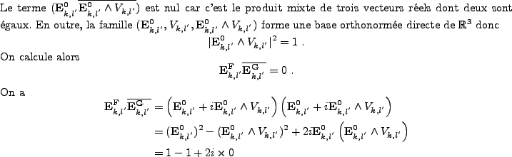
Un calcul élémentaire montre que l'on a la proposition 12 suivante.

Proposition 12   Les couples (<I>E^<I>F_k,l^',<I>H^<I>F_k,l^') et (<I>E^<I>G_k,l^',<I>H^<I>G_k,l^') vérifient les équations de Maxwell adjointes sans source dans $\Omega _k$, soit

$$\begin{array}{l} \mathop{{\mathbf {\nabla}} \wedge}\nolimits ... ...line{\varepsilon }_{k}{{\mathbf E}^{'}}= 0 \ . \\ \end{array}$$

Ces couples vérifient les relations de la définition de V_h (14) et permettent donc de définir l'espace de discrétisation V_h.

Proposition 13   Les conditions de la définition 15, soit,

$$% \left\{ \null\,\vcenter{\openup\jot \let\\ =\@ \ialign{\st... ...{'}},V_{k,l^{'}}) \in {\mathbb{R}}^2 \ , \cr \crcr}}\, \right.$$ (II.8.27)

impliquent

$${{\mathbf E}}^{{{\mathbf F}}}_{k,l^{'}} \overline{{{\mathbf E}}^{{{\mathbf G}}}_{k,l^{'}}} = 0 \ .$$ (II.8.28)

Cela signifie que, pour tout k de 1 à K et tout l^' de 1 à p, les fonctions <I>E^<I>F_k,l^' et <I>E^<I>G_k,l^' sont orthogonales dans ${\mathbb{C}}^3$ pour tout <I>X donné dans $\Omega _k$ donc dans ${{\mathcal{H}}}(\Omega_k,\partial \Omega_k)$.

Lemme 17   La famille (<I>E^<I>F_k,l,<I>E^<I>G_k,l)_l=1,p de cardinal L=2p est libre dans $\Omega _k$.